Mathematical models for predicting microstructural evolution

Research Overview
My research focus is on the microstructural coarsening of multicomponent multiphase polycrystalline materials during thermo-mechanical processes in the interdisciplinary areas of materials engineering. During my graduate studies (doctoral), I have been involved with the development of phase-field models and data-analytical tools to study several metallic/ceramic microstructural evolution processes. In particular, my doctoral dissertation (KIT, Germany) examines the underlying mechanisms responsible for grain coarsening in complex polycrystalline systems through large-scale 2-D and 3-D simulations. Besides, a considerable part of the thesis also explores the statistical quantification of the developing microstructures and their influence on growth phenomena using statistical tools like R. Before my doctoral research, I obtained my masters from IIT Madras, India in the area of specialization materials engineering.
Multi-Phase-field model
Microstructural evolution is thermodynamically driven by the minimization of free energy. Phase-field models: Implicit tracking of the interface movement is obtained through the formulation of partial differential equations. Bulk-free energy functions, related to specific material systems, can be derived from physical principles or can be computed from thermodynamic databases (CALPHAD).
Microstructural evolution of complex polycrystalline system \(\Rightarrow\) grand-potential formulation, \[\begin{equation} \label{gp1} \begin{split} \boldsymbol {\Omega} (T, \boldsymbol {\mu}, \boldsymbol {\phi}) & = \int_{V} \Big( \boldsymbol {\Psi}(T, \boldsymbol {\mu}, \boldsymbol {\phi})+ {\epsilon}{a}( \boldsymbol {\phi}, \boldsymbol {\nabla}\boldsymbol{\phi})+ \frac{1}{\epsilon}w( \boldsymbol {\phi}) \Big) \mathrm{d}{V} \end{split} \end{equation}\]
The gradient energy density,
\[\begin{equation} \label{c2gp3} \begin{split} {a}(\boldsymbol{\phi},\boldsymbol{\nabla}\boldsymbol{\phi}) & = \displaystyle\sum_{m<n} \sigma_{mn} {[a_{mn}(q_{mn})]}^{2} {|q_{mn}|}^{2} \end{split} \end{equation}\]
\[\begin{equation} \label{eq3} \begin{split} q_{mn} & = {\phi_{m} \boldsymbol{\nabla}{\phi}_{n}} - {\phi_{n} \boldsymbol{\nabla}{\phi}_{m}}. \end{split} \end{equation}\]
Multi-obstacle potential including higher order terms:
\[\begin{equation} \label{eq4} \begin{split} w(\boldsymbol{\phi}) & ={\frac{16}{{\pi}^{2}}} {\displaystyle\sum_{m<n} \sigma_{mn} \phi_{m} \phi_{n}}+ {\displaystyle\sum_{m<n} \sigma_{mno} \phi_{m} \phi_{n} \phi_{o}} \end{split} \end{equation}\]
Interpolation of the individual grand potential densities
\[\begin{equation} \label{eq13} \begin{split} \boldsymbol{\Psi} (T,\boldsymbol{\mu},\boldsymbol{\phi}) & = \displaystyle\sum_{\alpha=1}^{N} \Psi^{\alpha}(T,\boldsymbol{\mu}) h ({\phi}_{\alpha}) \end{split} \end{equation}\]
\[\begin{equation} \label{eq14} \begin{split} {\Psi}^{\alpha} (T,\boldsymbol{\mu}) & = f^{\alpha}(c^{\alpha}(\boldsymbol{\mu}),T) - \displaystyle\sum_{i=1}^{K-1} \mu_i c_i^{\alpha}(\boldsymbol{\phi},T) \end{split} \end{equation}\]
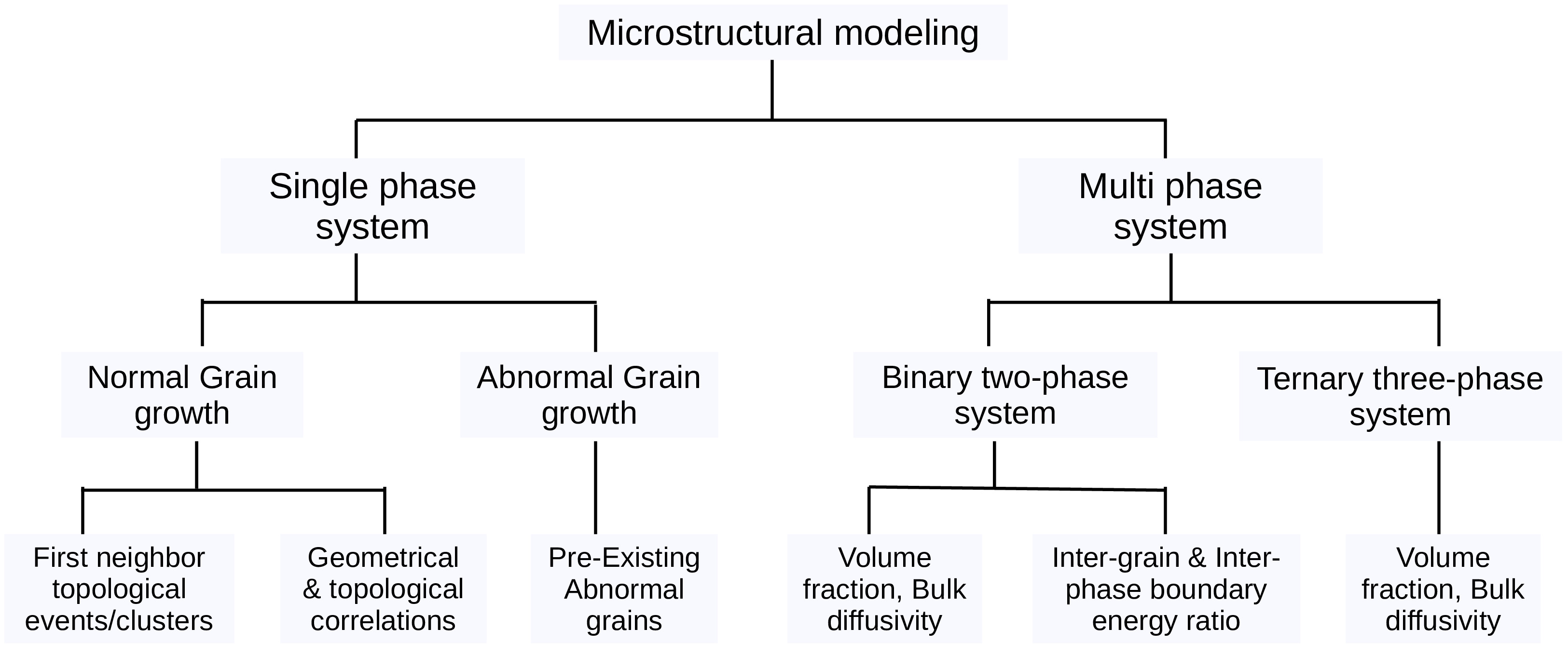
Binary two-phase system
The chemical energies of the respective phases are constructed using the parabolic type of functions: \[\begin{equation} \label{eq17} \begin{split} f^{\alpha} & = A_{\alpha}(c-c^{\alpha}_{eq})^2 \end{split} \end{equation}\]
\[\begin{equation} \label{eq18} \begin{split} f^{\beta} & = B_{\beta}(c-c^{\beta}_{eq})^2, \end{split} \end{equation}\]
The interpolated free energy as, \[\begin{equation} \label{eq16} \begin{split} f(\phi,c) & = f^{\alpha} h(\phi_\alpha)+f^{\beta} h(\phi_\beta), \end{split} \end{equation}\]
and where the coefficients of \(A_\alpha\) and \(B_\beta\) can be used to determine the steepness of the parabolic free energy. \(c^{\alpha}_{eq}\) and \(c^{\beta}_{eq}\) are the equilibrium compositions of the \(\alpha\) and \(\beta\) phase. \ The phase compositions will not deviate much from the equilibrium phase compositions in bulk materials.
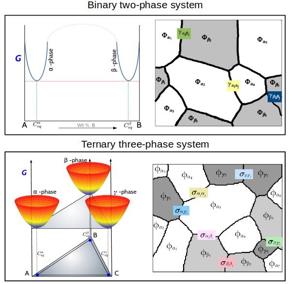
Ternary three-phase system
Three-phase polycrystalline structure which consists of a number of \(N(=N_{\alpha}+N_{\beta}+N_{\gamma})\), \(\alpha\), \(\beta\) and \(\gamma\) phase grains with different orientations. The chemical energies of the respective phases are constructed using the paraboloid type of functions:
where, \[\begin{multline*} f^{\alpha} (c_A,c_B,c_C) = \tilde{A}_{\alpha} c_{A}^{2} + \tilde{B}_\alpha c_{B}^{2} + \tilde{C}_\alpha c_{C}^{2} + \tilde{D}_\alpha c_A c_B \\ + \tilde{E}_\alpha c_B c_C + \tilde{F}_\alpha c_C c_A + \tilde{G}_\alpha c_A + \tilde{H}_\alpha c_B + \tilde{I}_\alpha c_C + \tilde{J}_\alpha , \end{multline*}\]
The \(\tilde{A}\), \(\tilde{B}\), \(\tilde{C}\), \(\tilde{D}\), \(\tilde{E}\), \(\tilde{F}\), \(\tilde{G}\), \(\tilde{H}\), \(\tilde{I}\) and \(\tilde{J}\) are the components at specific temperature. Taking the constraint \(c_A+c_B+c_C=1\), we can rearrange the above equation as follows. \[\begin{equation} \label{Eq0} \begin{split} f^{\alpha} &= A_{\alpha} (c_A-c_{A_\alpha}^{eq})^2 + B_{\alpha}(c_B-c_{B_\alpha}^{eq})^2 + C_\alpha \Big[(c_A-c_{A_\alpha}^{eq})(c_B-c_{B_\alpha}^{eq})\Big] + D_\alpha \end{split} \end{equation}\]
where \(c_A\), \(c_B\), \(c_C\) are the concentrations of A, B, and C, respectively.
The interpolated free energy as, \[\begin{equation} \begin{split} f(\phi,c) &= f^{\alpha} h(\phi_\alpha)+f^{\beta} h(\phi_\beta) +f^{\gamma} h(\phi_\gamma), \end{split} \end{equation}\]
Phase-field model (cont.)
The evolution equation for the conserved concentration fields can be expressed as follows: \[\begin{equation} \label{eq10} \begin{split} \frac{\partial{c_i}}{\partial t} &= \boldsymbol{\nabla} \cdot \Big( \displaystyle\sum_{j=1}^{K-1} M_{ij}(\boldsymbol{\phi}) \nabla \mu_j \Big). \end{split} \end{equation}\]
Here, \(M_{ij}(\boldsymbol{\phi})\) is the mobility of the interface, formulated as follows by an interpolation of the individual phase mobilities: \[\begin{equation} \label{eq11} \begin{split} M_{ij}(\boldsymbol{\phi}) &= \displaystyle\sum_{\alpha=1}^{N-1} M_{ij}^{\alpha} g_{\alpha} (\boldsymbol{\phi}). \end{split} \end{equation}\]
\[\begin{equation} \label{eq12} \begin{split} M_{ij}^{\alpha} &= D_{ij}^{\alpha} \Big(\frac{\partial c_{i}^{\alpha}(\boldsymbol{\mu},T)}{\partial \mu_j} \Big). \end{split} \end{equation}\]
The evolution equation for the nonconserved \(N\) phase-field variables \((\phi_{m},m=1,....,N)\) can be written as \[\begin{equation} \label{gp2} \begin{split} \tau \epsilon \frac{\partial {\phi_{m}}}{\partial t} & = \epsilon \Big[ \boldsymbol{\nabla} \cdot \frac{\partial a(\boldsymbol{\phi},\boldsymbol{\nabla}\boldsymbol{\phi})}{\partial \boldsymbol{\nabla}\phi_{m}}-\frac{\partial a(\boldsymbol{\phi},\boldsymbol{\nabla}\boldsymbol{\phi})}{\partial \phi_{m}} \Big]- \frac{1}{\epsilon} \frac{\partial w(\boldsymbol{\phi})}{\partial \phi_{m}}- \frac{\partial \boldsymbol{\Psi}(T,\boldsymbol{\mu},\boldsymbol{\phi})}{\partial{\phi}_m}- \lambda. \end{split} \end{equation}\]
Simulation set-up
The distribution of grains, in both 2D and 3D simulations, is implemented by a Voronoi algorithm wherein the points corresponding to the grains are randomly placed in the domain and allowed to initialize. A 3D representation of the final arrangements of the grains obtained by this algorithm is shown in the above Figure. In order to render an indicative statistical study, domains of sizes \(4000\times4000\) and \(512\times512\times512\) gridpoints with \(60000\) and \(75000\) grains are analysed in 2D and 3D, respectively. $ The variational derivative of the functional, \(\mathcal{F}\) with respect to the phase-field variable \(\phi_{\alpha}\) and phase-field gradient \(\boldsymbol{\nabla}\) \(\phi_{\alpha}\) generates scalar and vector respectively. Thus, an appropriate numerical scheme is adopted to optimize the evaluation . The evolution equation is discretized in an equidistant grid of cell sizes, \(\Delta\)x=\(\Delta\)y=\(\Delta\)z =1.0 by a finite difference method. A consistency within the simulations is attained by fixing the length scale of the diffuse interface width to \(\epsilon\)= 4\(\Delta\)x. Furthermore, simulations are made computationally efficient by implementing a which restricts the number of order parameters solved at each grid point.